Web GUI
The Ephemerista Web GUI provides an intuitive browser-based interface for satellite mission analysis. This manual guides you through all features and capabilities of the web application. The source code for the Web GUI is available at the LSF GitLab.
Getting Started
Installation and Setup
The Ephemerista Web GUI can be run using Docker or from source. The recommended approach is using the pre-built Docker image.
Download required data files:
Earth orientation parameters: finals2000A.all.csv
Planetary ephemerides: de440s.bsp
Orekit data package: orekit-data-main.zip
Place these files in a data directory (e.g.,
data/)Run the Docker container:
docker run -p 8000:8000 -v ./data:/app/backend/data registry.gitlab.com/librespacefoundation/ephemerista/ephemerista-web:latest
Open your browser and navigate to http://localhost:8000
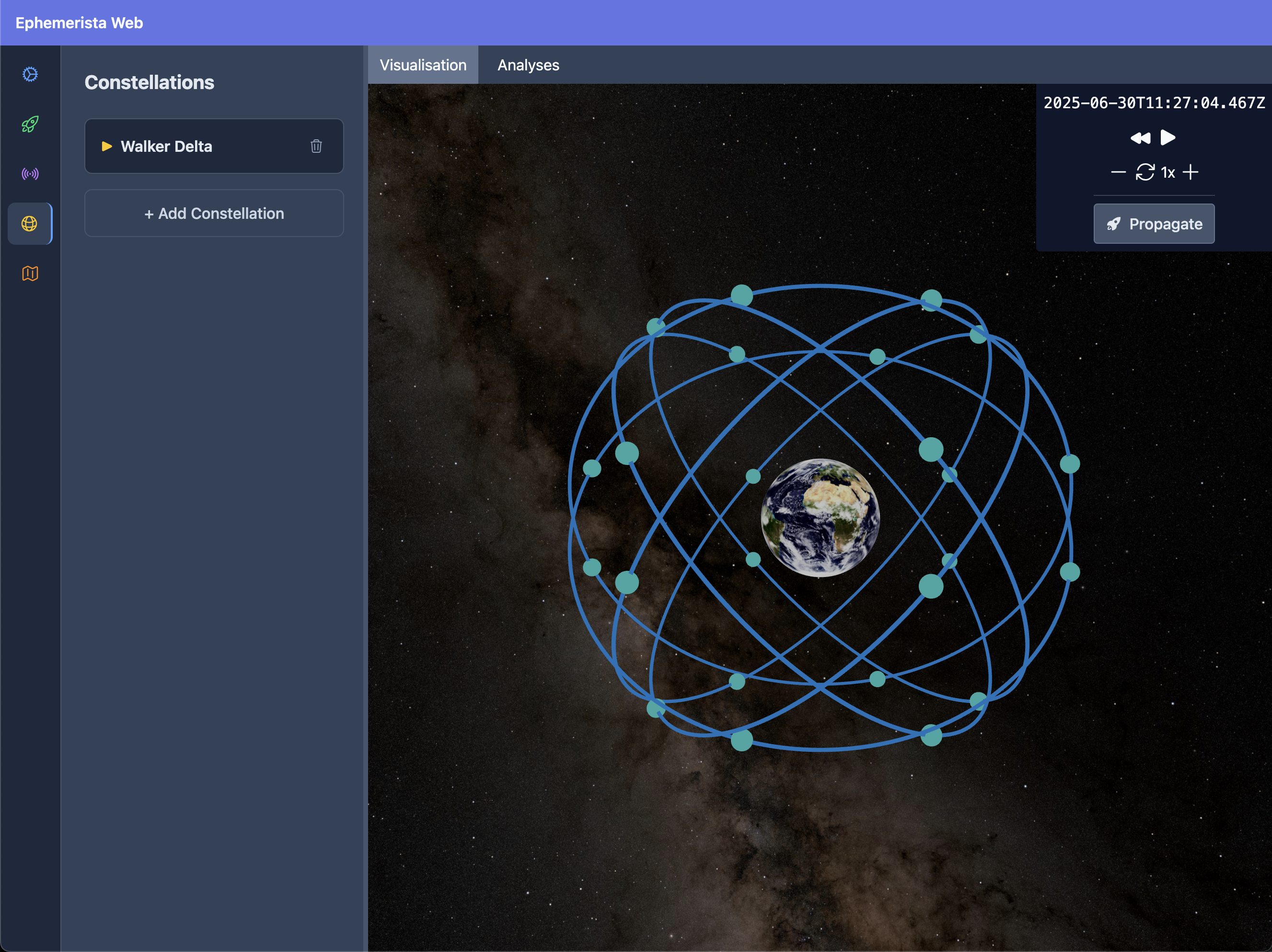
Main interface of the Ephemerista Web GUI
Interface Overview
The Ephemerista Web GUI consists of two main areas:
Left Sidebar: Resizeable navigation panel with vertical icon-based tabs and comprehensive form sections
Main Content Area: Dual-tab interface for visualization and analysis
Main Content Tabs
Visualisation Tab: Interactive 3D Earth viewer with orbital trajectories
Analyses Tab: Analysis configuration, execution, and results display
Creating Your First Scenario
Auto-Save Feature
The Ephemerista Web GUI automatically saves your work as you make changes:
Real-time Auto-Save: Changes are saved to browser local storage with a 1-second delay after editing
Visual Indicator: “Saving…” notification appears in the top-right corner during save
Persistent Storage: Your scenarios persist across browser sessions
No Manual Save Required: Focus on your analysis without worrying about losing work
Basic Scenario Setup
Scenario Information
Enter a descriptive name for your scenario
Set start and end times using the date/time pickers
Note: The web GUI only supports UTC timestamps
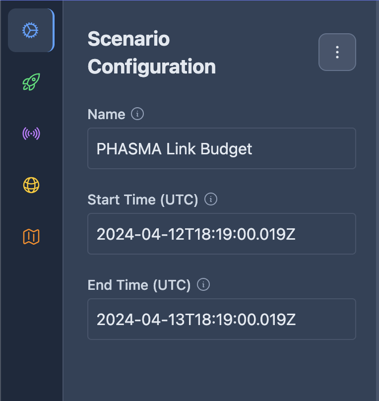
Scenario configuration panel
Adding Assets
Assets represent the spacecraft and ground stations in your mission. Click “Add Asset” to create new assets.
Spacecraft Configuration
Basic Information
Asset Name: Descriptive identifier
Asset Type: Select “Spacecraft”
Propagator Selection Choose how the spacecraft orbit will be calculated:
SGP4 Propagator (Recommended for TLE data)
Paste Two-Line Element (TLE) data
Default includes current ISS TLE for testing
Best for real satellite tracking
Numerical Propagator (High precision)
Initial state: Cartesian (position/velocity) or Keplerian elements
Force model configuration:
Gravity field degree and order (default: 4×4)
Third-body perturbations: Sun, Moon, planets
Solar radiation pressure (optional)
Atmospheric drag (optional)
Integrator settings: min/max step sizes, position error tolerance
Semi-analytical Propagator (Fast and accurate)
Same configuration options as Numerical
Faster computation using analytical methods
Good balance of speed and accuracy
OEM Propagator (Pre-computed orbits)
Upload CCSDS Orbit Ephemeris Message file
For precise, pre-calculated trajectories
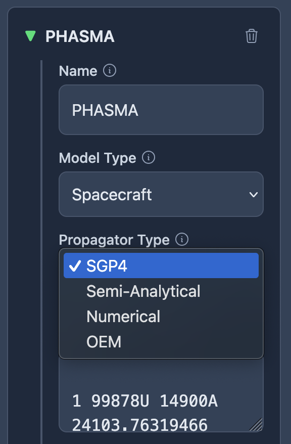
Propagator type selection
Initial State Configuration
For Cartesian States:
Position: X, Y, Z coordinates (km)
Velocity: VX, VY, VZ components (km/s)
Time: Initial epoch (UTC)
Reference frame: Coordinate system (ICRF default)
For Keplerian Elements:
Semi-major axis (km)
Eccentricity
Inclination (degrees)
Right ascension of ascending node (degrees)
Argument of periapsis (degrees)
True anomaly (degrees)
For Specialized Orbit Types:
The GUI provides simplified configuration for common orbital regimes:
LEO (Low Earth Orbit):
Altitude range: 160-2000 km
Inclination: 0-180 degrees
Common presets: ISS (~408 km), Starlink (~550 km)
Best for: Earth observation, communications
MEO (Medium Earth Orbit):
Altitude range: 2000-35786 km
Inclination: 0-180 degrees
Common preset: GPS (~20,200 km)
Best for: Navigation satellites, regional communications
GEO (Geostationary Earth Orbit):
Fixed altitude: 35,786 km
Longitude position: -180° to +180°
Optional inclination and eccentricity adjustments
Best for: Weather satellites, broadcast communications
SSO (Sun-Synchronous Orbit):
Altitude: 200-1500 km (typical range)
LTAN (Local Time of Ascending Node): 0-24 hours
Automatically calculates required inclination
Best for: Earth observation with consistent lighting
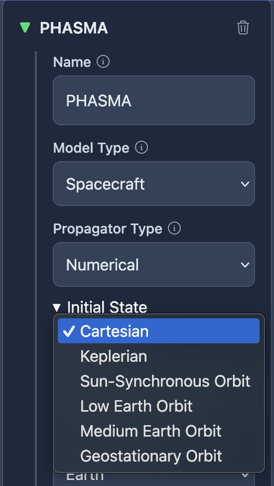
Initial state type selector
Ground Station Configuration
Geographic Location
Latitude: North/South position (degrees)
Longitude: East/West position (degrees)
Altitude: Height above sea level (meters)
Visibility Constraints
Minimum elevation: Lowest angle for visibility (degrees)
Typical values: 5-15° depending on terrain
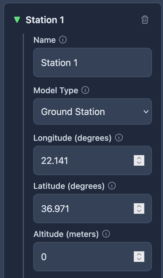
Ground station configuration
Communication Systems (Optional)
Configure communication systems for link budget analysis:
Channel Definition
Click “Add Channel” in the channels section
Configure channel parameters:
Link type: Uplink or Downlink
Data rate (bits/second)
Modulation: BPSK, QPSK, 8PSK, or QAM variants
Required Eb/N0 (dB)
System margin (dB)
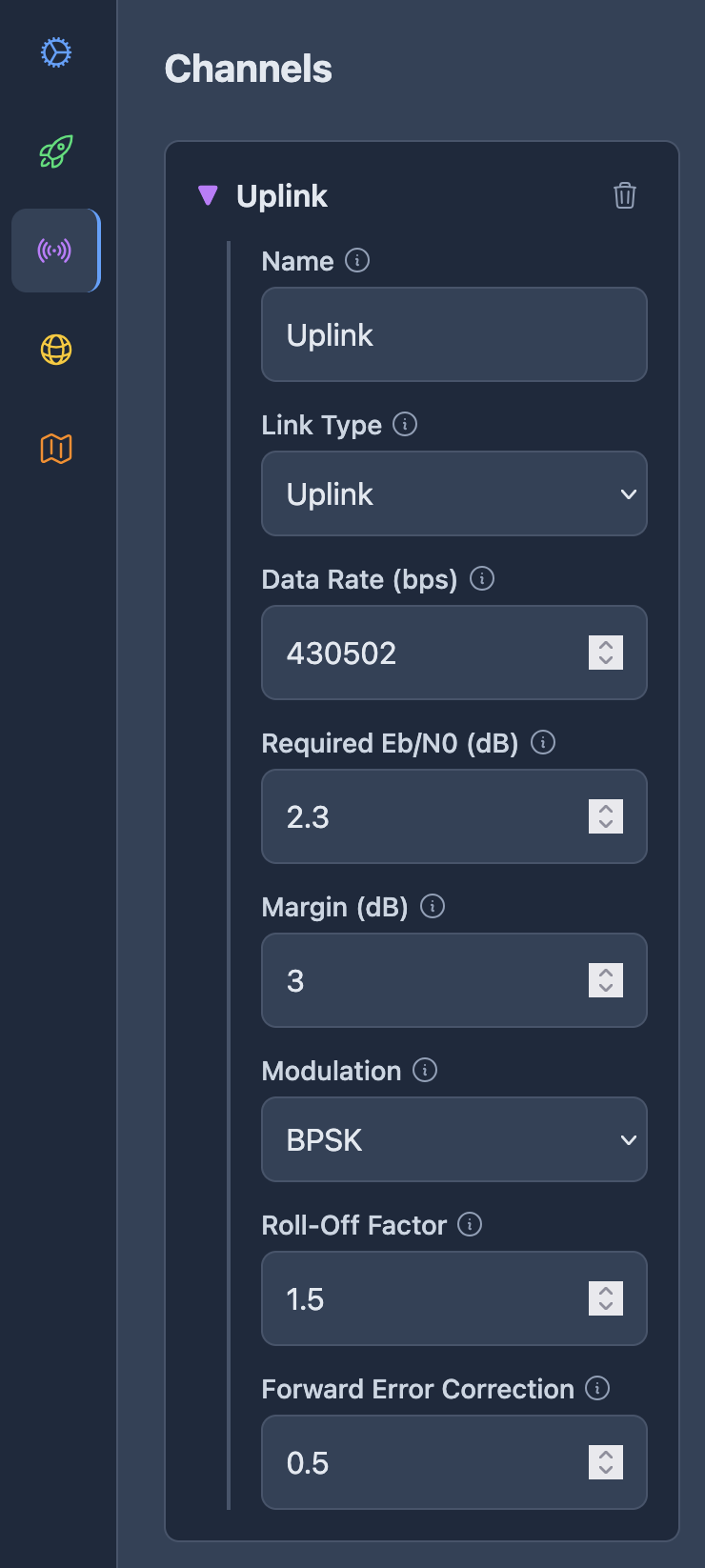
Communications channel configuration
Antenna Configuration
Add antennas to your assets for communication analysis:
Simple Antenna
Gain (dB): Antenna directivity
Beamwidth (degrees): Half-power beam width
Complex Antenna with Patterns
Parabolic: Diameter (m), efficiency (0-1)
Gaussian: Diameter (m), efficiency (0-1)
Dipole: Length (wavelengths)
MSI Pattern: Upload antenna pattern file
Transmitter/Receiver Setup
Transmitter
Output power (Watts)
Frequency (Hz)
Line losses (dB)
Receiver
System noise temperature (K) for simple receivers
Or detailed noise figure parameters for complex receivers
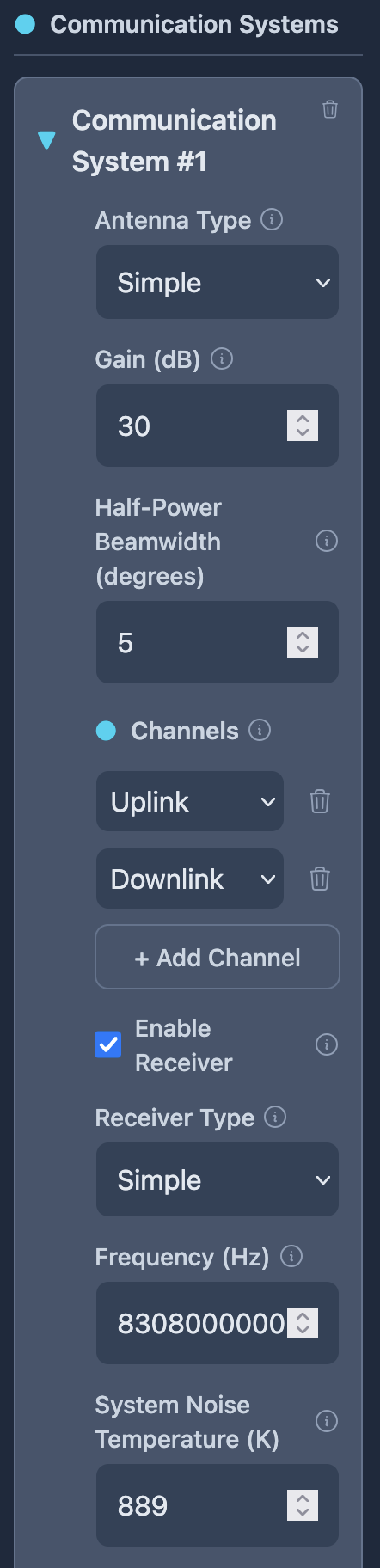
Communication system configuration
Constellations
Create large satellite constellations using predefined patterns:
Walker Constellations
Walker Delta (Traditional)
Number of satellites
Number of planes
Semi-major axis (km)
Inclination (degrees)
Phasing parameter
Walker Star (Rosette pattern)
Similar parameters to Walker Delta
Different phasing for improved coverage
Street of Coverage
Optimized for continuous coverage along specific latitude bands
J-parameter (Coverage Fold): 1-4, controls coverage redundancy
Best for: Global communications, continuous Earth observation
Flower Constellations
Petal Count: Number of petals in the flower pattern (1-20)
Days for Repeat Cycle: Ground track repetition period (1-30 days)
Number of Satellites: Total satellites in constellation
Phasing Parameters: Inter-satellite spacing control
Use Cases: Specialized coverage patterns, repeating ground tracks
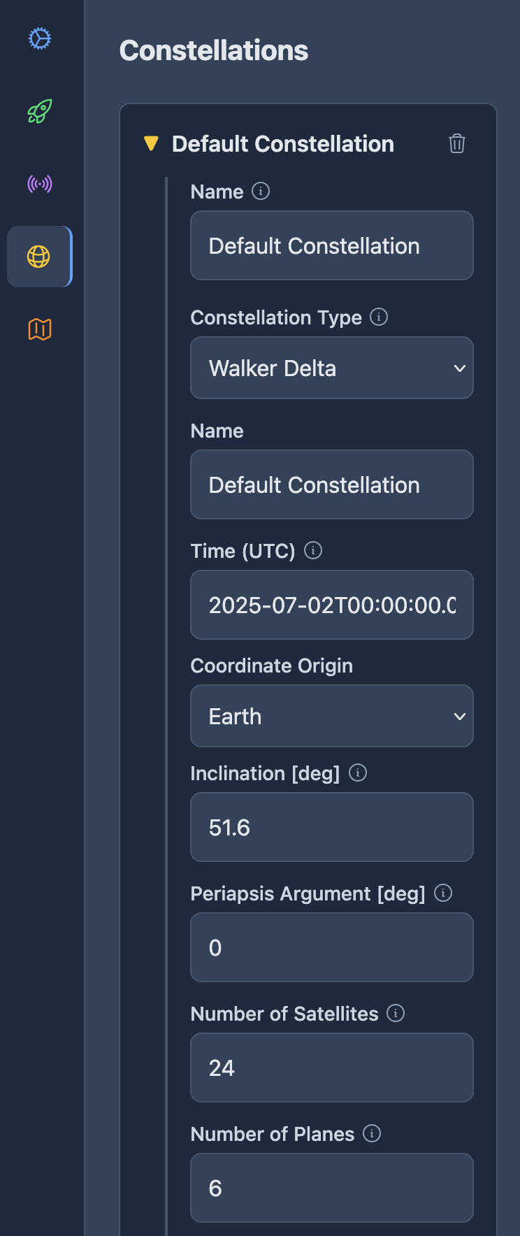
Constellation configuration
Asset Tracking Configuration
Ephemerista supports advanced antenna tracking where assets can automatically point their antennas toward other assets or constellation members. This feature is essential for maintaining communication links between spacecraft and ground stations.
Configuring Tracking in the GUI
In the Assets tab of the scenario configuration:
Navigate to Antenna Tracking Configuration: Found at the bottom of each asset’s configuration panel
Set Pointing Error: Define the tracking accuracy in degrees (typical values: 0.1° for high-precision systems, 0.5-1.0° for standard systems)
Select Tracked Assets: Choose individual assets from the list that this asset’s antennas should track
Select Tracked Constellations: Choose constellations to track any member spacecraft
Tracking configuration
Concurrent Access Handling
When multiple tracked assets are simultaneously visible and communicating with the tracking asset, Ephemerista currently assumes perfect tracking of all targets. This is physically impossible in reality, as a single antenna can only point at one target at a time. Future versions will implement prioritization logic to handle these scenarios more realistically by:
Selecting the highest priority target based on link margin, data rate, or user-defined criteria
Modeling switching time between targets
Accounting for lost communication during antenna repointing
Areas of Interest
Define geographic regions for coverage analysis:
Click “Add Area of Interest” in the Areas of Interest section
Use the interactive drawing tool to create rectangular areas on the map
Click “Draw Rectangle” and use click-and-drag to define the area
Configure area parameters:
Name: Descriptive identifier for the area
Minimum Elevation: Minimum satellite elevation angle (degrees)
Discretization: Grid resolution in degrees for coverage calculations
Save the drawn area
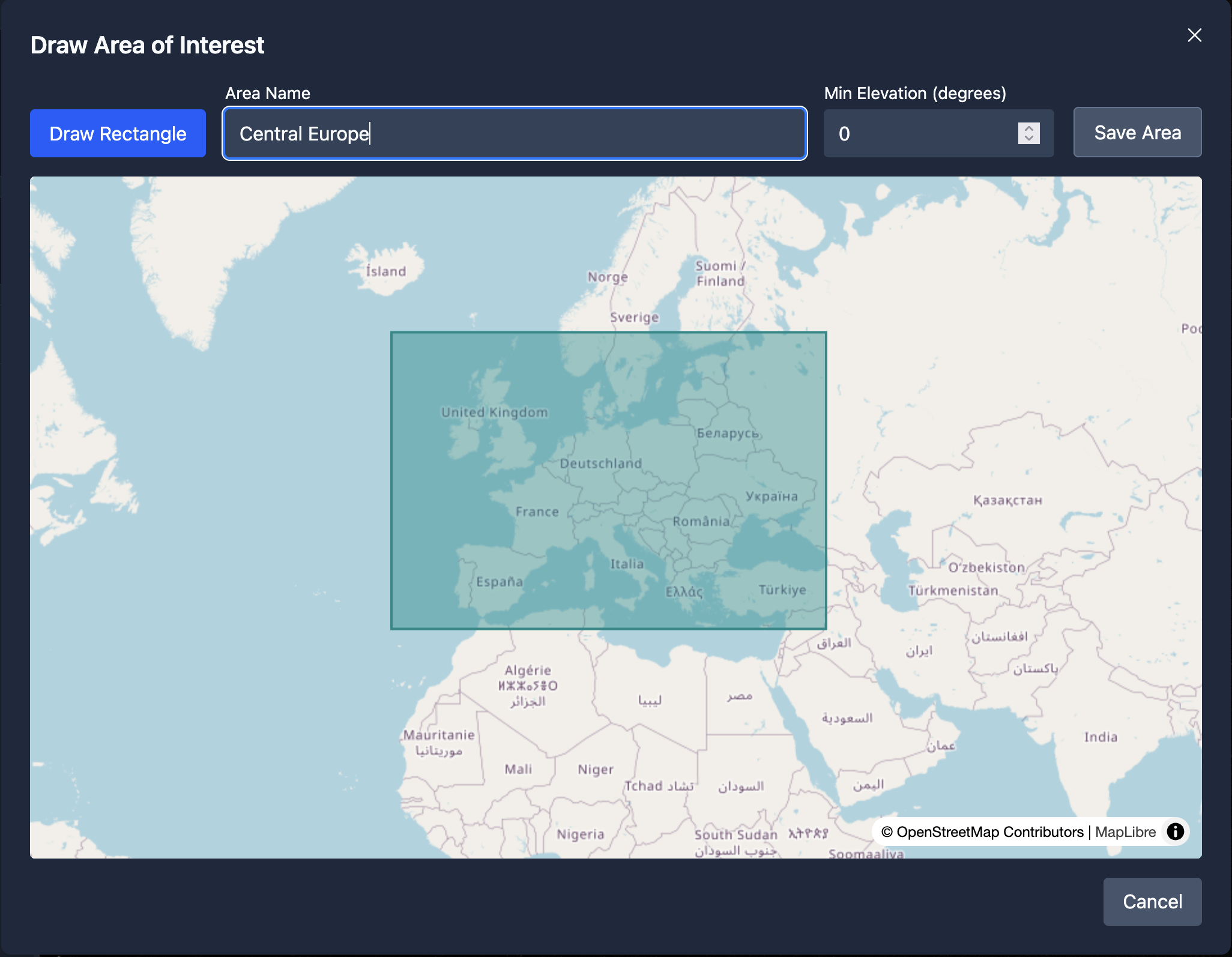
Drawing an area of interest of the map
Configuration Tips:
Discretization: Controls the grid resolution for coverage analysis
Smaller values (< 0.5°) provide more accurate results but slower computation
Larger values (1-2°) provide faster results suitable for initial analysis
Minimum Elevation: Typical values range from 5° to 15° depending on application
Multiple areas can be defined for comprehensive coverage analysis
Areas are saved with the scenario and can be edited later
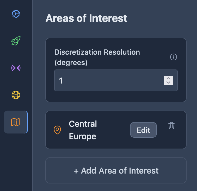
Area of interest configuration
Visualization
3D Earth Viewer
The main visualization shows an interactive 3D Earth with your mission assets:
Navigation Controls
Mouse drag: Rotate view around Earth
Mouse wheel: Zoom in/out
Asset Display
Spacecraft & constellations: Colored dots with orbital trails
Ground stations: Markers on Earth surface
Animation Controls
Play/Pause: Start/stop time progression
Speed Control: Adjust simulation speed (1x to 1000x)
Time Display: Current simulation time (UTC)
Propagation Controls
Propagate Button: Propagate and visualise orbits
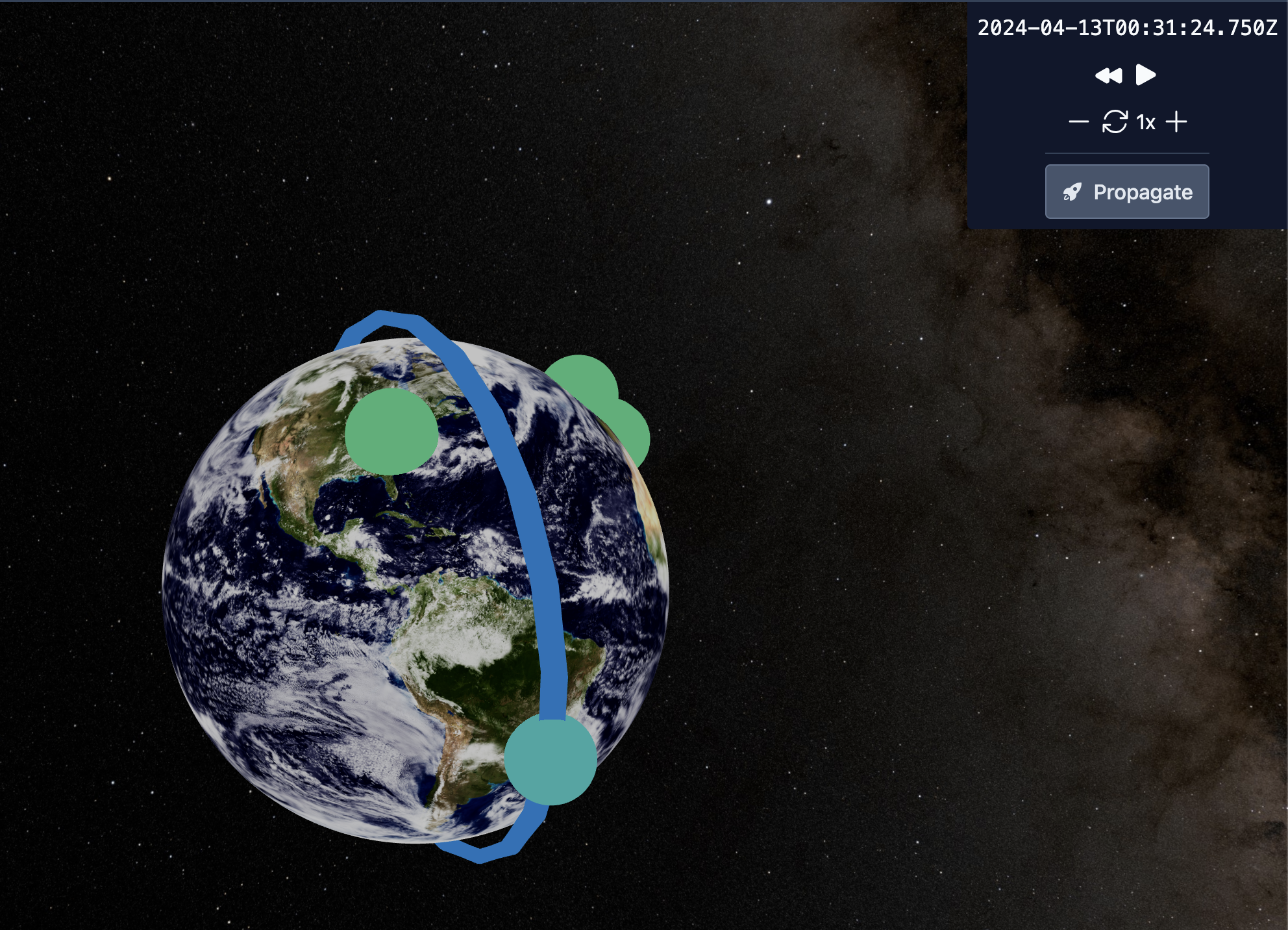
3D visualisation
Analysis Capabilities
Switch to the “Analyses” tab to perform mission analysis:
Visibility Analysis
Calculates when spacecraft are visible from ground stations.
Configuration
Select “Visibility” from analysis type dropdown
Choose observer (ground station) and target (spacecraft)
Click “Run Analysis”
Results
Pass Summary: List of all visibility passes
Pass Details: Individual pass characteristics
Visualization
Pass profile plots showing elevation and azimuth vs. time
Range and range rate profiles
Export Options
CSV files for specific observer-target pairs
Individual pass data
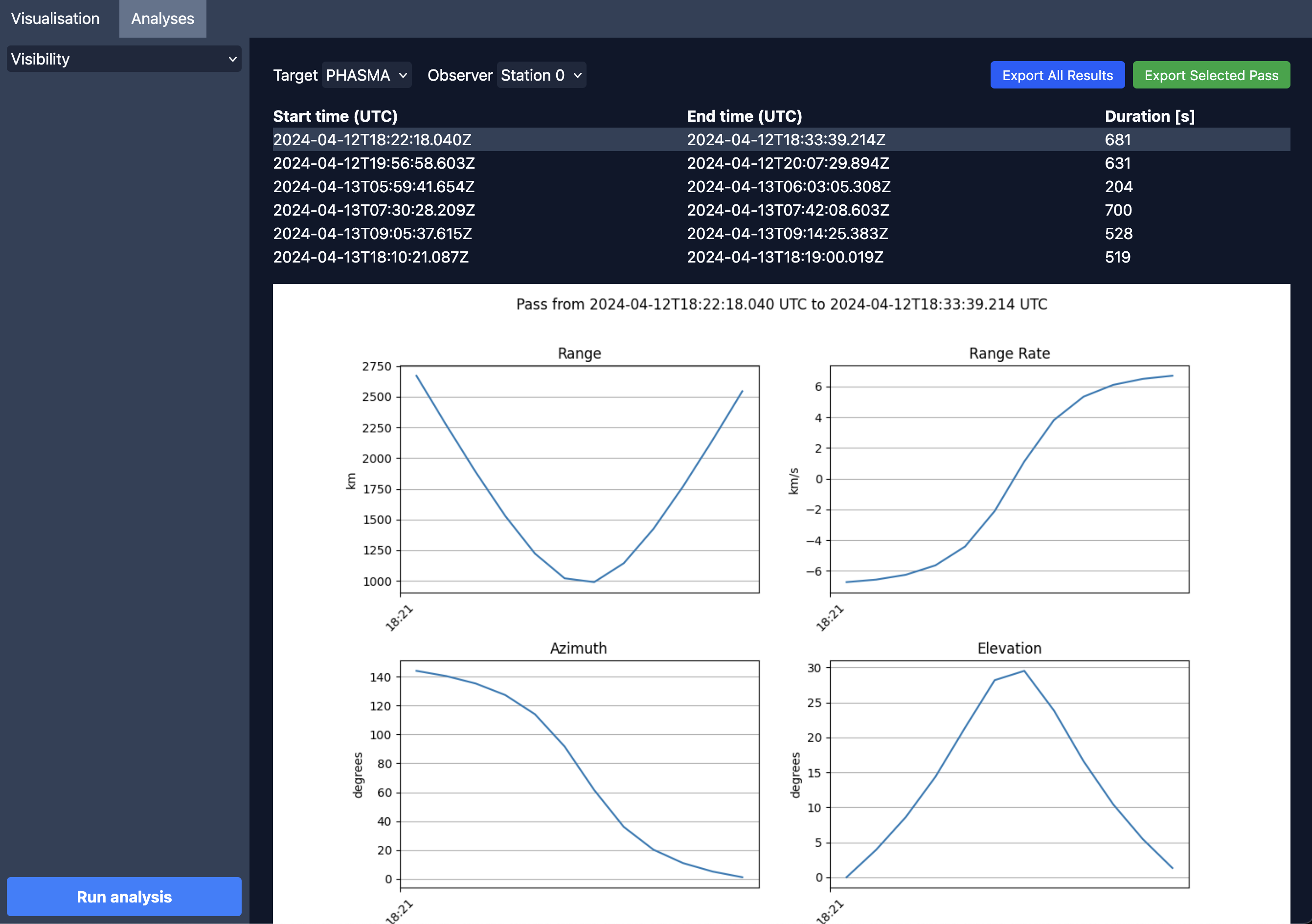
Visibility analysis
Link Budget Analysis
Evaluates communication link performance between assets.
Prerequisites
Assets must have communication systems configured
Channels must be defined
Antennas, transmitters, and receivers must be specified
Configuration
Select “Link Budget” from analysis type
Toggle interference analysis (if multiple transmitters)
Configure environmental loss models
Click “Run Analysis”
Results
Link Statistics:
EIRP (Effective Isotropic Radiated Power)
Path loss (Free space + atmospheric)
C/N0 (Carrier-to-noise ratio)
Eb/N0 (Energy per bit to noise ratio)
Link margin (dB)
Individual loss components
Plots
Link margin vs. time
Individual loss components
C/N0 and Eb/N0 profiles
Antenna pointing angles
Export Options
CSV Export Button: Available in the analysis results panel
Export Formats:
Pass Summary: Overview of all communication passes with key metrics
Individual Pass Data: Specific pass details with elevation/azimuth profiles
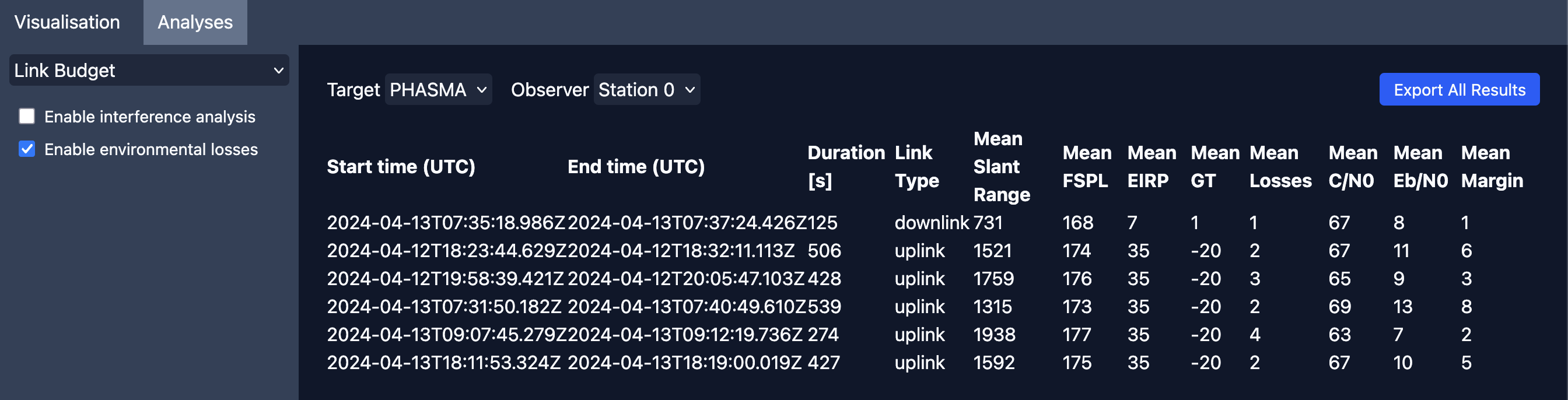
Link budget analysis
Navigation Analysis
Assesses GNSS-like navigation performance and positioning accuracy.
Prerequisites
Navigation constellation (e.g., GPS, Galileo, Glonass) with at least 4 satellites
Observer location (ground station or spacecraft)
Properly configured scenario timing
Configuration
Navigate to the “Analyses” tab in the main content area
Select “Navigation” from the analysis type dropdown
Set UERE (User Equivalent Range Error) parameter:
What it represents: Combined effect of all ranging error sources in meters
Typical values:
GPS (civilian): 5-7 meters
GPS (military P(Y)-code): 3-5 meters
Galileo: 3-5 meters
GLONASS: 5-10 meters
Multi-GNSS: 2-4 meters
Error sources included: Satellite clock errors, ephemeris errors, atmospheric delays, multipath, receiver noise
Impact: Position accuracy = DOP × UERE
Choose observer location from available ground stations
Click “Run Analysis”
Results and Metrics
DOP (Dilution of Precision) Values:
GDOP: Geometric Dilution of Precision (overall geometry quality)
PDOP: Position DOP (3D position accuracy)
HDOP: Horizontal DOP (latitude/longitude accuracy)
VDOP: Vertical DOP (altitude accuracy)
TDOP: Time DOP (clock bias accuracy)
Navigation Performance Metrics:
Position Accuracy Estimates: Expected error in meters
Service Availability: Percentage of time with adequate satellite geometry
Satellite Visibility: Number of visible satellites vs. time
Visualization Options
DOP Time Series: All DOP values plotted over the analysis period
Satellite Visibility Timeline: Count of visible satellites vs. time
Export Capabilities
DOP Statistics: Complete time series as CSV
Position Accuracy Timeline: Expected positioning performance over time
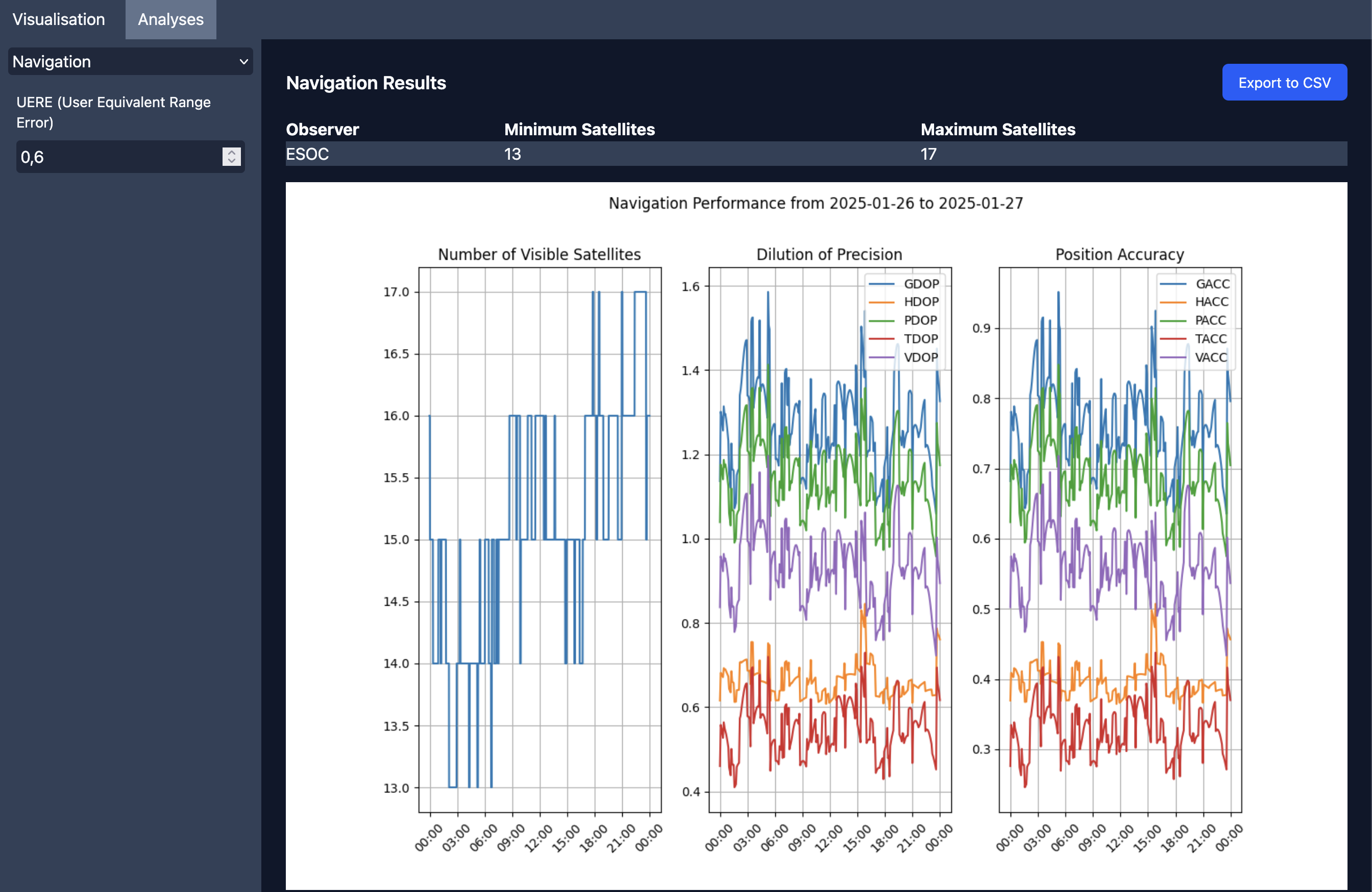
Navigation analysis
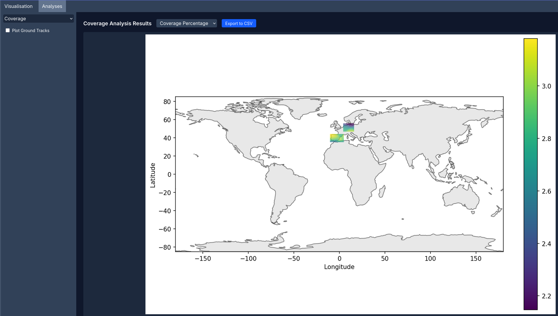
Coverage Analysis
Analyzes area coverage by satellite systems with comprehensive visualization and statistics.
Prerequisites
Areas of interest defined using the drawing tool
At least one satellite constellation or individual spacecraft
Properly configured scenario timing
Configuration
Define areas of interest with appropriate discretization:
In the Areas of Interest panel, set discretization in degrees for each area
1-2 degrees: Fast computation, good for initial analysis
0.5-1 degree: Balanced accuracy and speed
< 0.5 degrees: High accuracy, slower computation
Navigate to the “Analyses” tab in the main content area
Select “Coverage” from the analysis type dropdown
Select specific areas of interest to analyze (if multiple areas defined)
Select “Plot Ground Tracks” to print satellite Ground Tracks over the resulting map (make sure the Scene is propagated or analysis will fail to run)
Click “Run Analysis”
Results Display Options
The coverage analysis provides multiple visualization modes:
Coverage Percentage: Color-coded map showing percentage of time each area is covered and ground tracks if enabled
Time Gaps: Heat map displaying maximum time between successive coverage events
Statistics View: Detailed numerical results including:
Minimum, maximum, and average coverage percentages
Time gap statistics (min/max/average)
Total number of access events
Interactive Features
Area Selection: Click on specific areas to view detailed statistics
Export Capabilities
CSV Export: Complete coverage statistics for all areas
Area name and geometry (WKT format)
Coverage percentage
Time gap statistics (min/max/average in seconds and hours)
Number of discretized polygons
Access event count
Export Button: Click the CSV export button in the analysis results panel
Navigation analysis
Data Import and Export
Scenario Import/Export
Importing Scenarios
Click the dropdown arrow next to the scenario name in the header
Select “Import Scenario” from the dropdown menu
Choose your JSON scenario file
Review and modify the imported configuration as needed
Exporting Scenarios
Click the dropdown arrow next to the scenario name in the header
Select “Export Scenario” from the dropdown menu
Save the JSON file for future use or sharing with team members
Scenario File Format
JSON format with strict schema validation
Contains all asset, channel, and analysis configurations
Human-readable and editable in text editors
Compatible between different Ephemerista installations
Example Scenarios
Note
Pre-configured example scenarios are available for download to help you get started with Ephemerista.
Download Example Scenarios:
The Ephemerista repository includes several ready-to-use scenario files:
Lunar Transfer (405 KB): Lunar mission with multiple ground stations - Download
PHASMA Mission (8.3 KB): LEO satellite with link budget analysis - Download
PHASMA with Interference (10.6 KB): PHASMA scenario with interference sources - Download
Navigation (15 KB): GNSS constellation analysis - Download
Coverage (2.4 KB): Area coverage analysis scenario - Download
Using Example Scenarios:
Download a scenario JSON file from the links above
Click the dropdown arrow next to the scenario name in the web GUI header
Select “Import Scenario”
Choose the downloaded JSON file
The scenario will load with all assets, channels, and configurations pre-filled
These examples demonstrate various mission types and can serve as templates for your own scenarios.
Additional Example Data:
For more examples including Jupyter notebooks, antenna patterns, and GeoJSON areas, see the examples directory README.
Web GUI Limitations
The web interface provides an intuitive way to use Ephemerista but has some limitations compared to the full Python API:
Time System Constraints
UTC Only: Web GUI restricted to UTC timestamps
Python API Alternative: Use Time.from_components() with various time scales
Reference Frame Limitations
Earth-Centric Only: All coordinates relative to Earth
Python API Alternative: Support for all solar system bodies and barycenters
Advanced Configuration
Simplified Interface: Complex force models have preset options
Python API Alternative: Full programmatic control over all parameters
Batch Operations
Single Scenario Focus: One scenario at a time
Python API Alternative: Automated batch processing and parameter sweeps
Custom Analysis
Predefined Analysis Types: Four main analysis categories
Python API Alternative: Custom analysis workflows and algorithms
Help and User Assistance
Built-in Help System
The web GUI includes comprehensive contextual help to guide you through complex configurations:
Help Tooltips: Hover over the “?” icons next to form fields for detailed explanations
Orbital Mechanics Guidance: Tooltips include practical advice on parameter selection
Validation Feedback: Real-time validation with helpful error messages
Example Values: Common parameter ranges and typical mission values
User Interface Features
Auto-Complete: Form fields suggest common values and validate input ranges
Progress Indicators: Loading spinners show analysis progress
Toast Notifications: Success and error messages appear briefly in the corner
Consistent Styling: Uniform form layout across all configuration sections
Tips and Best Practices
Performance Optimization
Scenario Size
Start with small scenarios (< 10 assets) for testing
Large constellations (> 100 satellites) may take several minutes to propagate
Time Spans
Shorter analysis periods run faster
For initial testing, use 1-3 day periods
Extended coverage analysis may require 30+ days
Discretization Resolution
Coverage analysis: Start with resolution >1 deg
Increase resolution only after verifying scenario setup
Accurate Results
TLE Data Currency
Use recent TLE data for accurate tracking
TLEs degrade over time, especially for low Earth orbits
Ground Station Placement
Consider local terrain and obstructions
Use realistic minimum elevation angles (5-15°)
Communication System Modeling
Verify antenna patterns match hardware specifications
Include realistic system noise temperatures
Account for pointing losses and weather effects
Workflow Efficiency
Incremental Development
Start with simple scenarios and add complexity gradually
Use predefined orbit types (LEO, MEO, GEO, SSO) for initial setup
Test each component before adding the next
Take advantage of auto-save to experiment safely
Data Validation
Review propagated orbits in the 3D Visualisation tab
Check ground station visibility makes sense geographically
Verify communication coverage matches mission requirements
Use help tooltips to understand parameter impacts
Result Verification
Compare results across different analysis types
Cross-check with known mission parameters or benchmarks
Export data to CSV for detailed analysis in external tools
Use interactive visualization to explore edge cases
Troubleshooting
Common Issues
Scenario Won’t Load
Check JSON syntax if importing files
Verify all required fields are filled
Ensure date/time formats are valid
Analysis Fails
Verify all prerequisites are met:
Communication systems configured for link budget analysis
Areas of interest uploaded for coverage analysis
Sufficient satellites (4+) for navigation analysis
Check that orbital propagation completed successfully
Ensure scenario timing is properly configured
Review error messages in browser console (F12 → Console)
Auto-Save Issues
If auto-save stops working, refresh the browser tab
Check browser local storage permissions
Ensure stable internet connection for scenario persistence
Poor 3D Performance
Reduce number of visible orbital trails in visualization settings
Close other browser tabs to free up GPU memory
Use a recent browser version with WebGL 2.0 support
Disable browser extensions that might interfere with WebGL
Large File Uploads
Antenna pattern files: MSI files should be under 10MB for good performance
OEM files: Large ephemeris files may take time to process and validate
Interface Responsiveness
If the sidebar becomes unresponsive, try resizing it by dragging the edge
Clear browser cache if forms stop responding to input
Use the browser’s refresh function to reset the interface state
Getting Help
Built-in Help: Use the “?” tooltips throughout the interface for contextual guidance
Browser Console: Check for error messages (F12 → Console) if unexpected behavior occurs
Network Tab: Monitor API requests for debugging (F12 → Network)
Auto-Save Recovery: Your work is automatically saved, so refresh if the interface becomes unresponsive
Documentation: Refer to Python API docs for underlying concepts and advanced features
Example Scenarios: Start with simple configurations using predefined orbit types
Advanced Usage
Custom Antenna Patterns
Upload MSI (MATLAB Antenna Toolbox) pattern files for precise link budget analysis:
Generate antenna patterns using MATLAB Antenna Toolbox
Export as .pln file format (ensure compatibility)
Navigate to Complex Antenna configuration in the Assets section
Upload the pattern file - it will be automatically interpolated for analysis
Verify pattern import by reviewing the antenna gain visualization
OEM File Integration
Use pre-computed precise orbits for high-accuracy analysis:
Obtain CCSDS OEM (Orbit Ephemeris Message) file from mission planning tools
Select “OEM Propagator” in spacecraft configuration
Upload the OEM file - trajectory will be interpolated from ephemeris data
Suitable for high-precision mission analysis requiring cm-level accuracy
Verify ephemeris import by checking the orbital parameters display
Constellation Optimization
Design efficient satellite constellations:
Start with Walker or Street-of-Coverage patterns for global coverage
Use Flower constellations for specialized regional coverage
Adjust constellation parameters based on coverage analysis results
Export successful constellation configurations for reuse
Next Steps
Once you’re comfortable with the web GUI:
Export Results: Use CSV exports for detailed analysis in Excel or Python
Python API: Transition to programmatic analysis for complex workflows
Scenario Sharing: Share JSON scenario files with team members
Integration: Use web GUI for rapid prototyping, Python API for production analysis