Python API
This section provides detailed programming examples and concepts for using Ephemerista programmatically. The Python API offers full control over all features and advanced capabilities not available in the web GUI.
Quickstart
Installation
Ephemerista is distributed on PyPI and can be installed via pip.
# Create new virtual environment
python -m venv .venv
source .venv/bin/activate

# Install Ephemerista
pip install ephemerista
Obtain Required Data
Ephemerista requires the following data at runtime:
Earth orientation parameters from the IERS: finals2000A.all.csv
Planetary ephemerides in SPK format, e.g. de44s.bsp
An Orekit data package: orekit-data-main.zip
Alternatively, the Orekit data can be installed as a Python package via
pip, see here.
Initialise Ephemerista
Call the ephemerista.init function before using any other Ephemerista functionality and provide the paths to the required data files.
import ephemerista

EOP_PATH = ... # e.g. finals2000A.all.csv
SPK_PATH = ... # e.g. de440s.bsp
OREKIT_DATA_PATH = ... # e.g. orekit-data-main.zip

ephemerista.init(eop_path=EOP_PATH, spk_path=SPK_PATH, orekit_data=OREKIT_DATA_PATH)
If the Orekit data package was installed via package manager the orekit_data parameter can be omitted.
Use Ephemerista
Propagate the orbit of the ISS with Ephemerista.
import ephemerista
from ephemerista.propagators.sgp4 import SGP4
from ephemerista.time import TimeDelta

# Propgate the trajectory
iss_tle = """ISS (ZARYA)
1 25544U 98067A   24187.33936543 -.00002171  00000+0 -30369-4 0  9995
2 25544  51.6384 225.3932 0010337  32.2603  75.0138 15.49573527461367"""

propagator = SGP4(tle=iss_tle)
start_time = propagator.time
end_time = start_time + TimeDelta.from_hours(6)
times = start_time.trange(end_time, step=float(TimeDelta.from_minutes(1)))
trajectory = propagator.propagate(times)
Basics
This section demonstrates the fundamental concepts of Ephemerista, including trajectory propagation and ground track visualization. You’ll learn how to:
Propagate satellite orbits using TLE data
Create 3D trajectory visualizations
Generate ground track plots
Work with ground station networks
import plotly.graph_objects as go

import ephemerista
from ephemerista.assets import Asset, GroundStation
from ephemerista.plot.groundtrack import GroundTrack
from ephemerista.propagators.sgp4 import SGP4
from ephemerista.time import TimeDelta
## Propagate a trajectory
iss_tle = """ISS (ZARYA)
1 25544U 98067A   24187.33936543 -.00002171  00000+0 -30369-4 0  9995
2 25544  51.6384 225.3932 0010337  32.2603  75.0138 15.49573527461367"""

propagator = SGP4(tle=iss_tle)
start_time = propagator.time
end_time = start_time + TimeDelta.from_hours(6)
times = start_time.trange(end_time, step=float(TimeDelta.from_minutes(1)))
trajectory = propagator.propagate(times)
Plot 3D trajectory
fig = go.Figure()

fig.add_trace(trajectory.origin.plot_3d_surface())
fig.add_trace(trajectory.plot_3d())

fig.update_layout(
    title=f"3D trajectory, {trajectory.origin.name}-centered {trajectory.frame.abbreviation} frame",
)
fig.show()
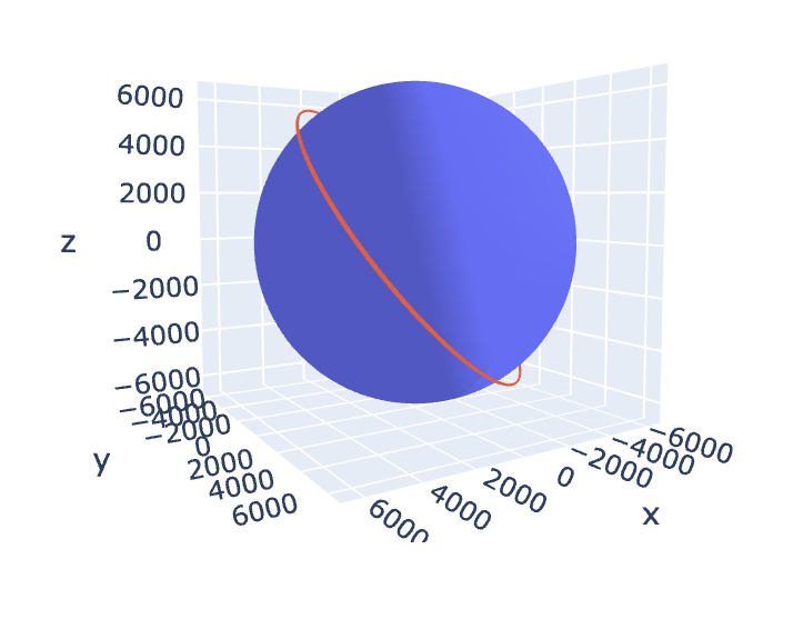
3D trajectory with Plotly
Plot ground track in 3D
#### Plot Spherical ground track
gt = GroundTrack(trajectory, label="ISS")
gt.plot()
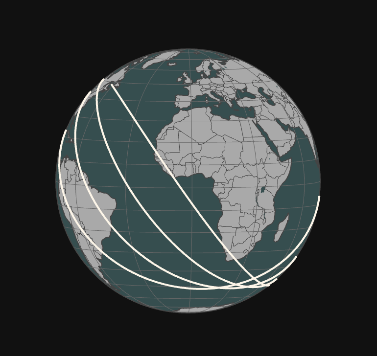
Ground track projected on a sphere
Plot classical ground track
## Change projection type
gt.update_projection("equirectangular")
gt.plot()
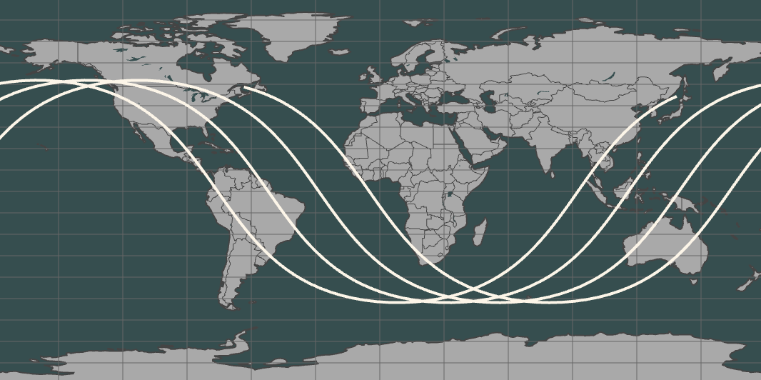
Classical ground track
Generate ground station network
station_data = [
    ("Kiruna", 67.858428, 20.966880),
    ("Esrange Space Center", 67.8833, 21.1833),
    ("Kourou", 5.2360, -52.7686),
    ("Redu", 50.00205516, 5.14518047),
    ("Cebreros", 40.3726, -4.4739),
    ("New Norcia", -30.9855, 116.2041),
]
stations = [Asset(model=GroundStation.from_lla(lon, lat), name=name) for name, lat, lon in station_data]
Add ground station to ground tracks
gt.plot_ground_station_network(stations)
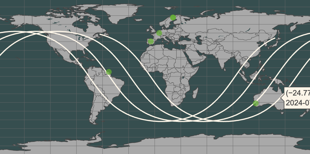
Ground track with ground station network
Orekit features
A certain number of features in ephemerista are based on the Orekit library, and in particular on its Jpype Python wrapper which was recently made available on PyPi.
Though available in Python, the Orekit Python wrapper interacts with a Java virtual machine in the background, therefore ephemerista also depends on a JDK, which is usually provided by jdk4py, available as a dependency of ephemerista.
Propagation
ephemerista’s NumericalPropagator and SemiAnalyticalPropagator inherit from the same base class, OrekitPropagator, because most of the code is similar between both. They are based on their Orekit counterparts, NumericalPropagator and DSSTPropagator:
The
NumericalPropagatoris a full-fledged numerical propagator based on a Dormand-Prince 8(5,3) variable step integrator, featuring most perturbation force models:Holmes-Featherstone gravitational model, up to an arbitrary degree and order.
Third-body attraction from any planet of the solar system, the Sun or the Moon
Solar radiation pressure, for now isotropic
Atmospheric drag based on the NRLMSISE00 density model, using three-hourly CSSI space weather data. For now isotropic.
The
SemiAnalyticalPropagatoruses the Orekit implementation of the Draper Semi-analytical Satellite Theory (DSST), which describes a semianalytical propagator that combines the accuracy of numerical propagators with the speed of analytical propagators. It features similar force models to theNumericalPropagator, and the Python parameters are the same.
Initialization
The propagator’s initial state vector must be provided as a TwoBody object, either in Keplerian or in Cartesian representation.
From Cartesian (position, velocity)
import numpy as np

from ephemerista.coords.twobody import Cartesian
from ephemerista.time import Time

time_start = Time.from_iso("TDB", "2016-05-30T12:00:00")

r = np.array([6068.27927, -1692.84394, -2516.61918])  # km
v = np.array([-0.660415582, 5.495938726, -5.303093233])  # km/s

state_init = Cartesian.from_rv(time_start, r, v)
From Keplerian
from ephemerista.angles import Angle
from ephemerista.coords.anomalies import TrueAnomaly
from ephemerista.coords.shapes import RadiiShape
from ephemerista.coords.twobody import Inclination, Keplerian
from ephemerista.time import Time

time_start = Time.from_iso("TDB", "2016-05-30T12:00:00")

state_init = Keplerian(
    time=time_start,
    shape=RadiiShape(ra=10000.0, rp=6800.0),  # km
    inc=Inclination(degrees=98.0),
    node=Angle(degrees=0.0),
    arg=Angle(degrees=0.0),
    anomaly=TrueAnomaly(degrees=90.0),
)
Propagator Configuration
The propagator takes at least the initial state as parameter. The initial state can later be overriden though by calling the method set_initial_state.
Declaring a simple propagator with default parameters, in either the numerical or the semi-analytical flavour:
from ephemerista.propagators.orekit.numerical import NumericalPropagator

propagator = NumericalPropagator(state_init=state_init)
from ephemerista.propagators.orekit.semianalytical import SemiAnalyticalPropagator

propagator = SemiAnalyticalPropagator(state_init=state_init)
The following float arguments can be passed to the NumericalPropagator or SemiAnalyticalPropagator constructors for general configuration of the propagators:
prop_min_step: Minimum integrator step, default is 1 millisecond. Referenceprop_max_step: Maximum integrator step, default is 3600 seconds. Referenceprop_init_stepInitial integrator step, default is 60 seconds. Referenceprop_position_error: Order of magnitude of the desired position error of the integrator for a sample LEO orbit, default is 10 meters. Decreasing this value can improve the propagation accuracy for complex force models, but will slow down the propagator. Referencemass: spacecraft mass in kilograms, default is 1000 kilograms.
Force model configuration
Without any arguments passed to the constructor, the default force model uses Earth spherical harmonics up to degree and order 4. As both the NumericalPropagator and SemiAnalyticalPropagator use the same arguments, in the following we will show only examples with the NumericalPropagator.
Loading a custom gravity model
Only the 4 file formats supported by Orekit are available in ephemerista. For instance to load a ICGEM file:
from pathlib import Path

propagator = NumericalPropagator(state_init=state_init, gravity_file=Path("ICGEM_GOCO06s.gfc"))
The following example configures gravity spherical harmonics with degree and order 64.
propagator = NumericalPropagator(state_init=state_init, grav_degree_order=(64, 64))
The following disables the spherical harmonics to only keep a Keplerian model.
propagator = NumericalPropagator(state_init=state_init, grav_degree_order=None)
Third-body perturbations
The following adds the Sun as a third-body perturbation.
from ephemerista.bodies import Origin

propagator = NumericalPropagator(state_init=state_init, third_bodies=[Origin(name="Sun")])
The following adds the Sun, the Moon and Jupiter as third-body perturbators.
propagator = NumericalPropagator(
    state_init=state_init, third_bodies=[Origin(name="Sun"), Origin(name="luna"), Origin(name="jupiter")]
)
Solar radiation pressure
Simply use the enable_srp flag, which is False by default.
Use cross_section to set the spacecraft cross-section in m^2 and c_r to set the reflection coefficient. Reference
propagator = NumericalPropagator(state_init=state_init, enable_srp=True, cross_section=0.42, c_r=0.8)
Atmospheric drag
Simply use the enable_drag flag, which is False by default.
Use cross_section to set the spacecraft cross-section in m^2 and c_d to set the drag coefficient. Reference
propagator = NumericalPropagator(state_init=state_init, enable_drag=True, cross_section=0.42, c_d=2.1)
Full-fledged force model
propagator = NumericalPropagator(
    state_init=state_init,
    mass=430.5,
    cross_section=0.42,
    c_d=2.1,
    c_r=0.8,
    grav_degree_order=(64, 64),
    third_bodies=[Origin(name="Sun"), Origin(name="luna"), Origin(name="jupiter")],
    enable_srp=True,
    enable_drag=True,
)
Propagator usage
Propagating to a single date
To perform a single propagation to a date:
time_end = Time.from_iso("TDB", "2016-05-30T12:01:00")

state_end = propagator.propagate(time=time_end)
Propagating from a list of Time
To retrieve all the intermediary state vectors between the initial and the final states, pass a list of Time objects to the propagator’s propagate method via the time argument:
time_end = Time.from_iso("TDB", "2016-05-30T16:00:00")
t_step = 60.0  # s
time_list = time_start.trange(time_end, t_step)

trajectory = propagator.propagate(time=time_list)
Stopping conditions
It is possible to stop propagation at events defined in the enum ephemerista.propagators.events.StoppingEvent. As of now, apoapsis and periapsis can be used as stopping conditions. The example below shows how to stop the propagation at periapsis. The same can be done for the apoapsis using the enum value StoppingEvent.APOAPSIS instead of StoppingEvent.PERIAPSIS.
from ephemerista.angles import Angle
from ephemerista.coords.anomalies import TrueAnomaly
from ephemerista.coords.shapes import RadiiShape
from ephemerista.coords.twobody import Inclination, Keplerian
from ephemerista.propagators.events import StoppingEvent
from ephemerista.time import Time

time_start = Time.from_iso("TDB", "2016-05-30T12:00:00")

state_init = Keplerian(
    time=time_start,
    shape=RadiiShape(ra=10000.0, rp=6800.0),  # km
    inc=Inclination(degrees=98.0),
    node=Angle(degrees=0.0),
    arg=Angle(degrees=0.0),
    anomaly=TrueAnomaly(degrees=90.0),
)

time_end = Time.from_iso("TDB", "2016-05-30T14:00:00")
t_step = 60.0  # s
time_list = time_start.trange(time_end, t_step)

propagator.set_initial_state(state_init)
trajectory = propagator.propagate(time=time_list, stop_conds=[StoppingEvent.PERIAPSIS])
CCSDS OEM/OPM/OMM import/export
ephemerista is able to read and write CCSDS OEM, OPM and OMM messages among others.
Writing CCSDS OEM files
ephemerista supports writing CCSDS files in both KVN and XML formats, relying on Orekit in the background.
from ephemerista.propagators.orekit.ccsds import CcsdsFileFormat, write_oem

dt = 300.0
write_oem(trajectory, "oem_example_out.txt", dt, CcsdsFileFormat.KVN)
write_oem(trajectory, "oem_example_out.xml", dt, CcsdsFileFormat.XML)
Reading CCSDS OEM files
from ephemerista.propagators.orekit.ccsds import parse_oem

dt = 300.0
trajectory = parse_oem("OEMExample5.txt", dt)
Visibility
Visibility analysis determines when spacecraft are visible from ground stations. This section covers:
Setting up visibility scenarios
Computing visibility windows (passes)
Analyzing pass characteristics (elevation, azimuth, duration)
Visualizing visibility results
import ephemerista
from ephemerista.analysis.visibility import Visibility
from ephemerista.scenarios import Scenario
scenario = Scenario.load_from_file("../tests/resources/lunar/scenario.json")
visibility = Visibility(scenario=scenario)
results = visibility.analyze()
This runs the analysis and returns results that can be further processed or visualized.
sc = scenario["Lunar Transfer"]
gs = scenario["CEBR"]
# Returns a table of passes for a specific observer/target combination
results.to_dataframe(gs, sc)
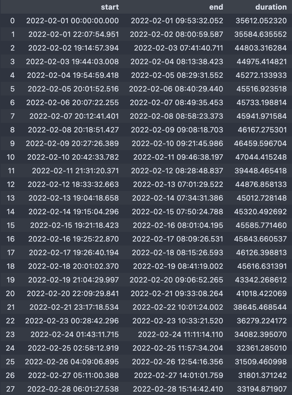
Visibility results
We can also plot the statistics for a single pass.
passes = results[gs, sc]
passes[2].plot()
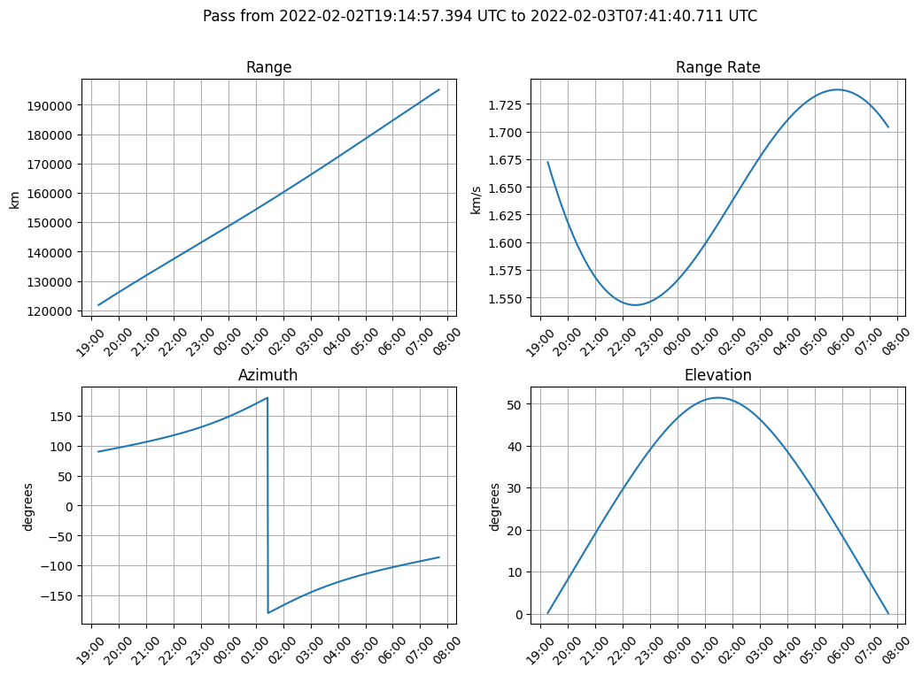
A single ground station pass
Antenna Tracking Configuration
Ephemerista supports antenna tracking of specific assets or constellations.
import ephemerista
from ephemerista import Scenario
from ephemerista.assets import Asset, GroundStation, Spacecraft
from ephemerista.constellation.design import Constellation, WalkerDelta
from ephemerista.time import Time, TimeDelta

## Create ground stations
gs1 = Asset(
    name="Ground Station 1",
    model=GroundStation.from_lla(longitude=-77.0, latitude=39.0)
)
gs2 = Asset(
    name="Ground Station 2",
    model=GroundStation.from_lla(longitude=2.3, latitude=48.8)
)

## Create spacecraft
from ephemerista.propagators.sgp4 import SGP4
tle = """SATELLITE
1 25544U 98067A   24001.00000000  .00000000  00000+0  00000+0 0    09
2 25544  51.6400   0.0000 0000000   0.0000   0.0000 15.50000000    00"""
sc = Asset(
    name="Spacecraft",
    model=Spacecraft(propagator=SGP4(tle=tle))
)

## Create scenario with assets
start_time = Time.from_iso("TDB", "2024-01-01T00:00:00")
end_time = start_time + TimeDelta.from_days(1)
scenario = Scenario(
    name="Tracking Demo",
    start_time=start_time,
    end_time=end_time,
    assets=[gs1, gs2, sc]
)

## Configure tracking
## Method 1: Direct asset tracking
gs1.track(asset_ids=[sc.asset_id])  # Ground station tracks spacecraft
sc.track(asset_ids=[gs1.asset_id, gs2.asset_id])  # Spacecraft tracks multiple ground stations

## Method 2: Constellation tracking
## Create a constellation
walker = WalkerDelta(
    time=start_time,
    nsats=6,
    nplanes=2,
    inclination=55.0,
    semi_major_axis=7000.0
)
constellation = Constellation(name="Demo Constellation", model=walker)

## Create a new scenario with the constellation
scenario_with_constellation = Scenario(
    name="Tracking Demo with Constellation",
    start_time=start_time,
    end_time=end_time,
    assets=[gs1, gs2],
    constellations=[constellation]
)

## Ground stations track any constellation member
gs1.track(constellation_ids=[constellation.constellation_id])
gs2.track(constellation_ids=[constellation.constellation_id])

## Set tracking accuracy
gs1.pointing_error = 0.5  # degrees
gs2.pointing_error = 0.5
sc.pointing_error = 0.1  # Higher precision for spacecraft
Antennas
This section focuses on antenna modeling for communication analysis. You’ll learn about:
Different antenna types and patterns
Gain calculations and beam modeling
Antenna pointing and coverage
Integration with communication systems
Note
For the polar plots the \(\theta\) angle (i.e. corresponding to the elevation) is in the [0, 360°] range. This is only for the polar plots, in reality the \(\theta\) angle is in the [0, 180°] range, or [-90, 90°] or in the [0, 90°] depending on the \(\theta\)/\(\phi\) conventions for parametrizing antenna patterns.
As of now, all antennas depend only on the \(\theta\) angle and are \(\phi\)-invariant. However, this might change in the future when new antenna types are introduced.
We first define two orbits that will be used later for 3D cones and contour plots.
from ephemerista.propagators.sgp4 import SGP4

iss_tle = """ISS (ZARYA)
1 25544U 98067A   24187.33936543 -.00002171  00000+0 -30369-4 0  9995
2 25544  51.6384 225.3932 0010337  32.2603  75.0138 15.49573527461367"""

iss_prop = SGP4(tle=iss_tle)
c_iss = iss_prop.propagate(iss_prop.time)

geo_tle = """EUTELSAT 36D
1 59346U 24059A   24317.58330181  .00000165  00000+0  00000+0 0  9993
2 59346   0.0146 287.8797 0000094 214.1662 156.0172  1.00269444  2311"""
geo_prop = SGP4(tle=geo_tle)
c_geo = geo_prop.propagate(geo_prop.time)
import plotly.graph_objects as go
Parabolic antenna
We define a parabolic antenna of 75cm diameter, 60% efficiency. We first use this antenna at 8.4 GHz (X band).
freq_parabol = 8.4e9
from ephemerista.comms.antennas import ComplexAntenna, ParabolicPattern
parabolic_antenna = ComplexAntenna(pattern=ParabolicPattern(diameter=0.75, efficiency=0.6))
Polar pattern diagram
fig = go.Figure()

fig.add_trace(parabolic_antenna.plot_pattern(frequency=freq_parabol))

fig.update_layout(
    title="Antenna pattern diagram (polar) [dBi]", polar={"angularaxis": {"rotation": 90, "direction": "clockwise"}}
)
fig.show()
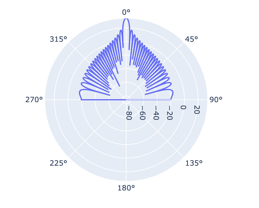
Polar parabolic antenna pattern
Linear pattern diagram
fig = go.Figure()
fig.add_trace(parabolic_antenna.plot_pattern(frequency=freq_parabol, fig_style="linear"))
fig.update_layout(title="Antenna pattern diagram (cartesian) [dBi]", xaxis_range=[-90.0, 90.0])
fig.show()
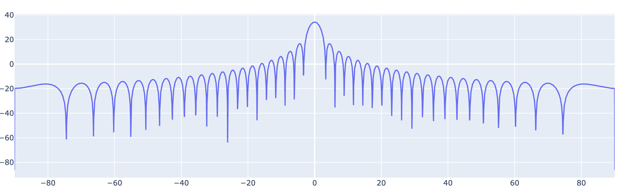
Linear parabolic antenna pattern
Contour Map Plots
ISS orbit, X band
geomap = parabolic_antenna.plot_contour_2d(frequency=freq_parabol, sc_state=c_iss)
display(geomap)
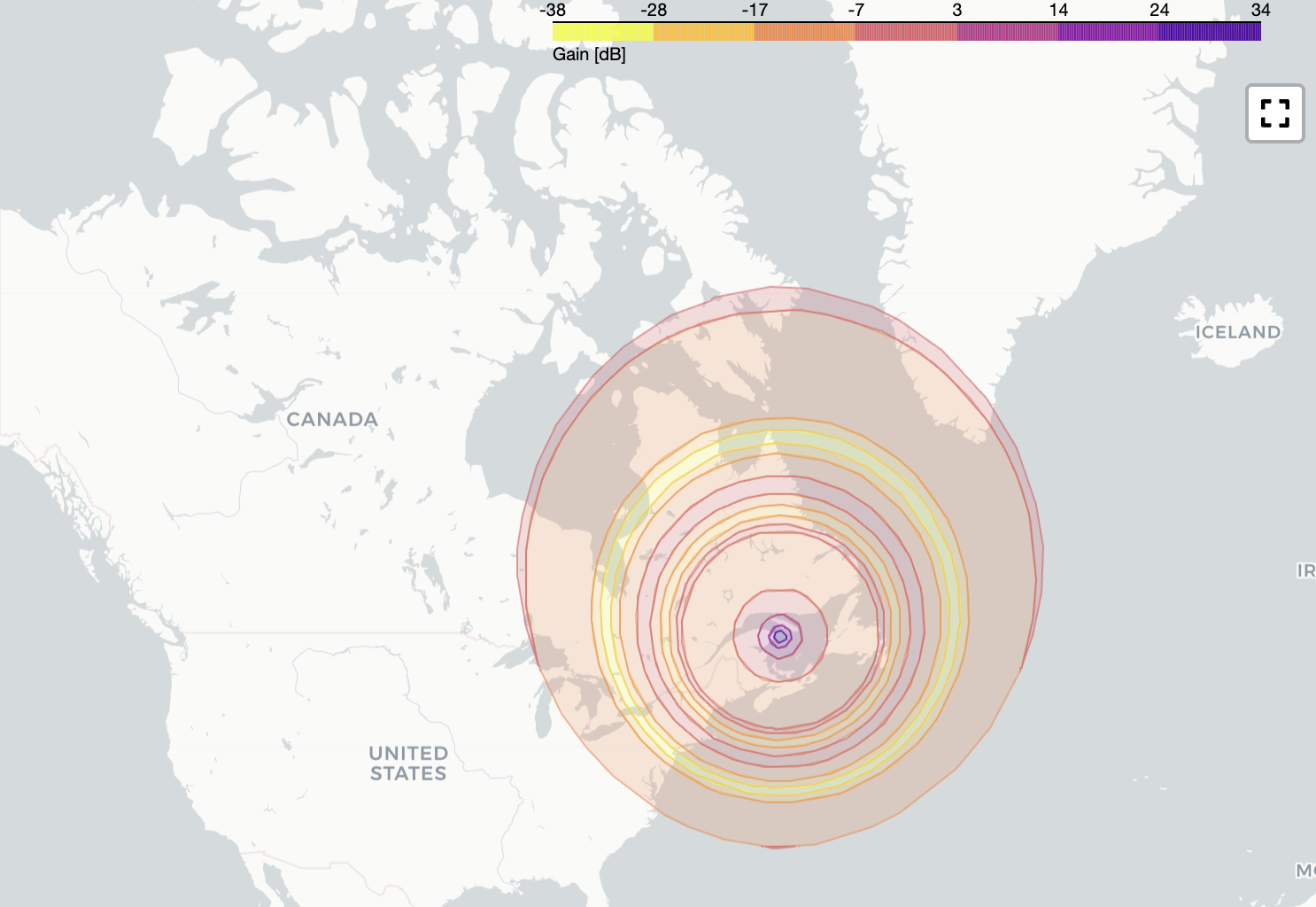
Contour plot ISS X band
ISS orbit, Ka band
geomap = parabolic_antenna.plot_contour_2d(frequency=31e9, sc_state=c_iss)
display(geomap)
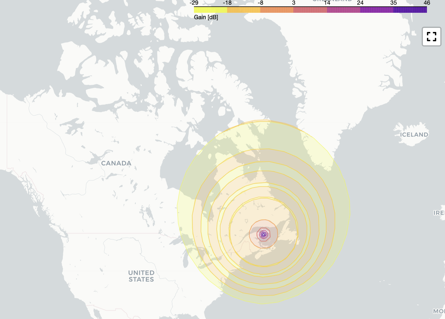
Contour plot ISS Ka band
Geostationary satellite, Ka band
geomap = parabolic_antenna.plot_contour_2d(frequency=31e9, sc_state=c_geo)
display(geomap)
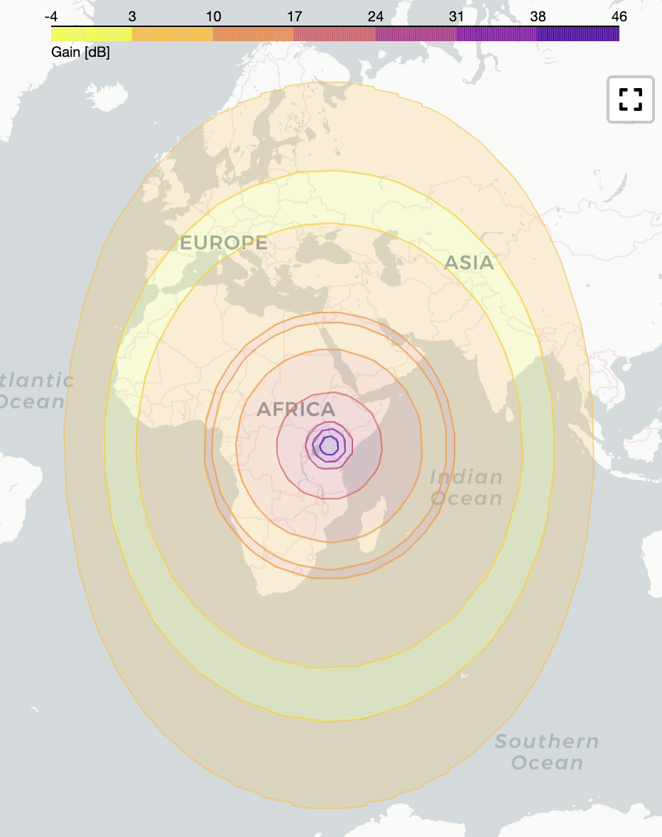
Contour plot geostationary Ka band
Dipole antennas
freq_dipole = 433e6
from ephemerista.comms.antennas import DipolePattern
from ephemerista.comms.utils import wavelength
Half wavelength vs short dipole: polar pattern diagrams
dipole_halfwavelength = ComplexAntenna(
    pattern=DipolePattern(length=wavelength(frequency=freq_dipole) / 2), boresight_vector=[0, 1, 0]
)
dipole_short = ComplexAntenna(pattern=DipolePattern(length=wavelength(frequency=freq_dipole) / 1000))
fig = go.Figure()
fig.add_trace(dipole_halfwavelength.plot_pattern(frequency=freq_dipole, trace_name="Half wavelength"))
fig.add_trace(dipole_short.plot_pattern(frequency=freq_dipole, trace_name="Short dipole"))

fig.update_layout(
    title="Antenna pattern diagram (polar) [dBi]",
    polar={"radialaxis": {"range": [-12.0, 3.0]}, "angularaxis": {"rotation": 90, "direction": "clockwise"}},
)
fig.show()
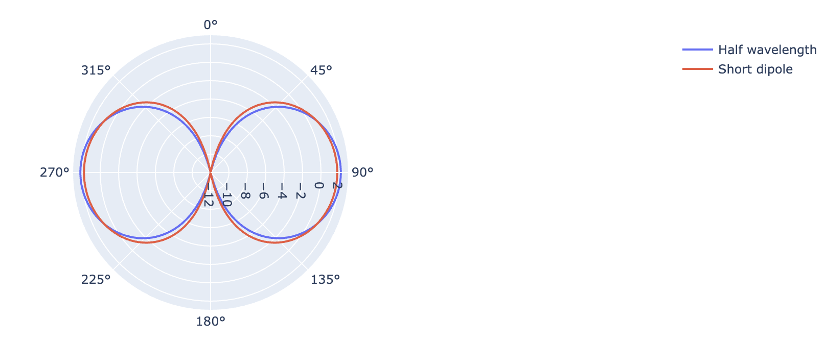
Polar dipole antenna pattern
3D visibility cone
The following cell shows 2 visibility cones corresponding to the following frequencies and satellites:
A parabolic antenna at 8.4 GHz from a geostationary satellite, pointed towards nadir
A parabolic antenna at 2.2 GHz from the ISS, pointed towards the velocity vector
from ephemerista.plot.utils import ensure_3d_cube_aspect_ratio

fig = go.Figure()

planet_mesh3d = c_geo.origin.plot_3d_surface()
fig.add_trace(planet_mesh3d)

cone_viz_geo = parabolic_antenna.viz_cone_3d(frequency=8.4e9, sc_state=c_geo, opacity=0.5, name="GEO sat")
fig.add_trace(cone_viz_geo)
fig.add_trace(
    go.Scatter3d(x=[c_geo.position[0]], y=[c_geo.position[1]], z=[c_geo.position[2]], name="GEO sat", mode="markers")
)

parabol_towards_velocity = ComplexAntenna(
    pattern=ParabolicPattern(diameter=0.75, efficiency=0.6), boresight_vector=[1, 0, 0]
)
cone_viz_iss = parabol_towards_velocity.viz_cone_3d(
    frequency=2.2e9, sc_state=c_iss, opacity=0.5, name="ISS", cone_length=20000
)
fig.add_trace(cone_viz_iss)
fig.add_trace(
    go.Scatter3d(x=[c_iss.position[0]], y=[c_iss.position[1]], z=[c_iss.position[2]], name="ISS", mode="markers")
)

fig.update_layout(
    title="Antenna cone 3D visualization",
    autosize=False,
    width=1000,
    height=700,
)

ensure_3d_cube_aspect_ratio(fig)

fig.show()
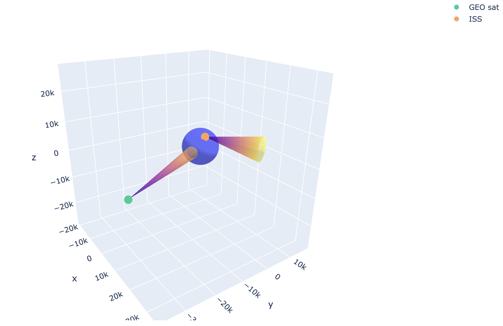
3D cones
MSI Import
For more complex antenna patterns Ephemerista supports the import of MSI Planet files.
from pathlib import Path

from ephemerista.comms.antennas import MSIPattern

msi_file = Path("..") / "tests" / "resources" / "antennas" / "cylindricalDipole.pln"
pattern = MSIPattern.read_file(msi_file)
antenna = ComplexAntenna(pattern=pattern)

fig = go.Figure()
fig.add_trace(ComplexAntenna(pattern=pattern).plot_pattern(frequency=pattern.frequency, trace_name="MATLAB"))
fig.add_trace(
    ComplexAntenna(pattern=DipolePattern(length=2.0)).plot_pattern(
        frequency=pattern.frequency, trace_name="Ephemerista"
    )
)

fig.update_layout(
    title="Antenna pattern diagram (polar) [dBi]",
    polar={"radialaxis": {"range": [-20.0, 6.0]}, "angularaxis": {"rotation": 90, "direction": "clockwise"}},
)
fig.show()
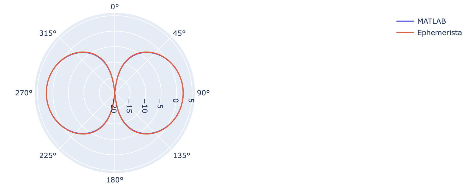
MSI Planet antenna pattern from MATLAB compared to the Ephemerista implementation
Link budgets
Link budget analysis evaluates the performance of RF communication links. This section demonstrates:
Communication system setup
Link budget calculations (with or without interference)
Performance metrics (EIRP, path loss, environmental losses, margin)
import ephemerista
from ephemerista.analysis.link_budget import LinkBudget
from ephemerista.angles import Angle
from ephemerista.assets import Asset, GroundStation, Spacecraft
from ephemerista.comms.antennas import SimpleAntenna
from ephemerista.comms.channels import Channel
from ephemerista.comms.receiver import SimpleReceiver
from ephemerista.comms.systems import CommunicationSystem
from ephemerista.comms.transmitter import Transmitter
from ephemerista.propagators.sgp4 import SGP4
from ephemerista.scenarios import Scenario
from ephemerista.time import TimeDelta
Link budget without interference
uplink = Channel(link_type="uplink", modulation="BPSK", data_rate=430502, required_eb_n0=2.3, margin=3)
downlink = Channel(link_type="downlink", modulation="BPSK", data_rate=861004, required_eb_n0=4.2, margin=3)
## S-Band
frequency = 8308e6  # Hz
gs_antenna = SimpleAntenna(gain_db=30, beamwidth_deg=5, design_frequency=frequency)
gs_transmitter = Transmitter(power=4, frequency=frequency, line_loss=1.0)
gs_receiver = SimpleReceiver(system_noise_temperature=889, frequency=frequency)
gs_system = CommunicationSystem(
    channels=[uplink.channel_id, downlink.channel_id],
    transmitter=gs_transmitter,
    receiver=gs_receiver,
    antenna=gs_antenna,
)
sc_antenna = SimpleAntenna(gain_db=6.5, beamwidth_deg=60, design_frequency=frequency)
sc_transmitter = Transmitter(power=1.348, frequency=frequency, line_loss=1.0)
sc_receiver = SimpleReceiver(system_noise_temperature=429, frequency=frequency)
sc_system = CommunicationSystem(
    channels=[uplink.channel_id, downlink.channel_id],
    transmitter=sc_transmitter,
    receiver=sc_receiver,
    antenna=sc_antenna,
)
station_coordinates = [
    (38.017, 23.731),
    (36.971, 22.141),
    (39.326, -82.101),
    (50.750, 6.211),
]

stations = [
    Asset(
        model=GroundStation.from_lla(longitude, latitude, minimum_elevation=Angle.from_degrees(10)),
        name=f"Station {i}",
        comms=[gs_system],
    )
    for i, (latitude, longitude) in enumerate(station_coordinates)
]
tle1 = """
1 99878U 14900A   24103.76319466  .00000000  00000-0 -11394-2 0    01
2 99878  97.5138 156.7457 0016734 205.2381 161.2435 15.13998005    06
"""

propagator1 = SGP4(tle=tle1)
sc1 = Asset(model=Spacecraft(propagator=propagator1), name="PHASMA", comms=[sc_system])
Set all ground stations to track the spacecraft, and set the spacecraft to track the first ground station.
Note
If no tracking is specified, the antenna’s boresight vector is used for computing pattern angle losses (in LVLH frame for a spacecraft, and in topocentric frame for a ground station).
## Configure tracking - each ground station tracks the spacecraft
for station in stations:
    station.track(asset_ids=[sc1.asset_id])

## Spacecraft tracks the first ground station
sc1.track(asset_ids=[stations[0].asset_id])
start_time = propagator1.time
end_time = start_time + TimeDelta.from_days(1)

scenario1 = Scenario(
    assets=[*stations, sc1],
    channels=[uplink, downlink],
    name="PHASMA Link Budget",
    start_time=start_time,
    end_time=end_time,
)
Showing the overview of the ground station passes as a dataframe.
lb = LinkBudget(scenario=scenario1)
results = lb.analyze()
results.to_dataframe(stations[0], sc1)

Link budget results table
Showing plots between the first ground station and the spacecraft. As both are tracking each other, both the TX and the RX angles are always 0.
results[stations[0], sc1][0].plot()
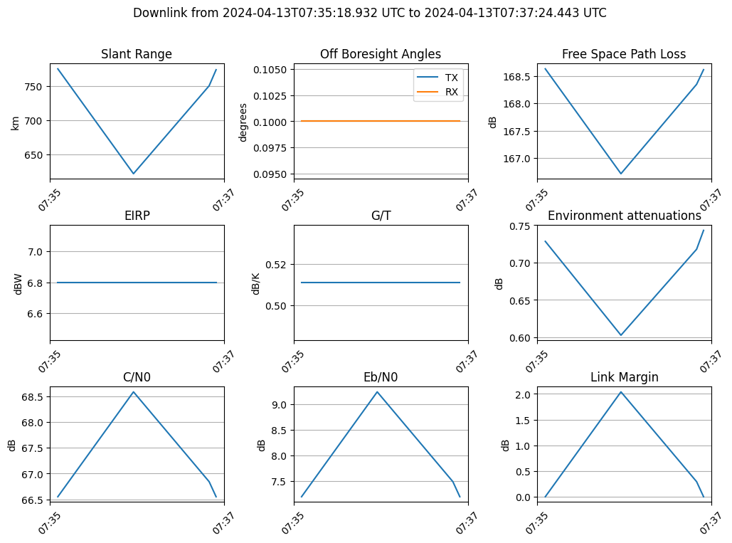
Plotted results for a single link
Environmental losses
Environmental losses are included in the link budget if the with_environmental_losses flag is enabled. They are computed using the itur Python library based on the ITU-R recommendations. The following losses are included:
Link budget with interference analysis
Adding a nearby spacecraft to the scenario to demonstrate downlink interference.
As the scenario already contains several ground stations close to each other, there will be uplink interference too.
The interference calculations are based on a MATLAB example:
First, the contact times are computed and it is checked if the interference sources are visible from the target asset in the considered time window
Then the overlapping portion of the target’s signal bandwidth with the bandwidth of the interferers is computed.
The overlap factor computed above allows to calculate the amount of power from the interferers that acts as interference within the target’s signal bandwidth
The new performance figures
C/(I0+N0)andEb/(I0+N0)are computed in the same way as the interference-free figuresC/N0andEb/N0, but with the interference power added to the noise powerThese new performance figures allow computing the new link margin which is reduced by the interference.
tle2 = """
1 99878U 14900A   24103.76319466  .00000000  00000-0 -11394-2 0    01
2 99878  97.5138 156.7457 0016734 205.2381 191.2435 15.13998005    09
"""

propagator2 = SGP4(tle=tle2)
sc2 = Asset(model=Spacecraft(propagator=propagator1), name="INTERFERER", comms=[sc_system])

scenario2 = Scenario(
    assets=[*stations, sc1, sc2],
    channels=[uplink, downlink],
    name="PHASMA Link Budget with interference",
    start_time=start_time,
    end_time=end_time,
)

lb2 = LinkBudget(scenario=scenario2, with_interference=True)
results_with_interference = lb2.analyze()
Here is the same link budget but with interference.
results_with_interference[stations[0], sc1][idx_pass].plot(plot_interference=True)
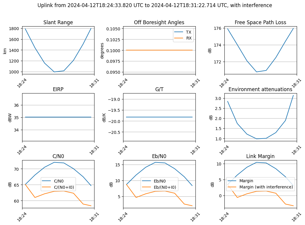
Plotted results for a single link with interference
Constellations & Coverage Analysis
Constellation design is crucial for providing global coverage. This section covers:
Walker constellation patterns
Street-of-Coverage designs
Coverage analysis
Walker Star Constellation
from ephemerista.constellation.design import StreetOfCoverage, WalkerStar
from ephemerista.time import Time, TimeDelta

constel = WalkerStar(
    time=Time.from_iso("TDB", "2016-05-30T12:00:00"),
    nsats=18,
    nplanes=6,
    semi_major_axis=7000,
    inclination=45,
    eccentricity=0.0,
    periapsis_argument=90,
)
First we inspect the planes of the constellation.
constel.to_dataframe()
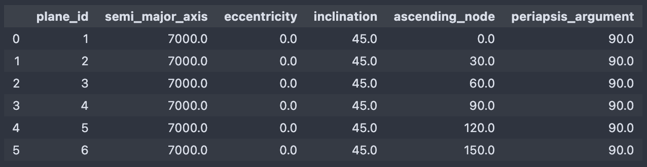
The planes of the Walker star constellation
And then the individual satellites of the constellation.
constel.to_dataframe("satellites")
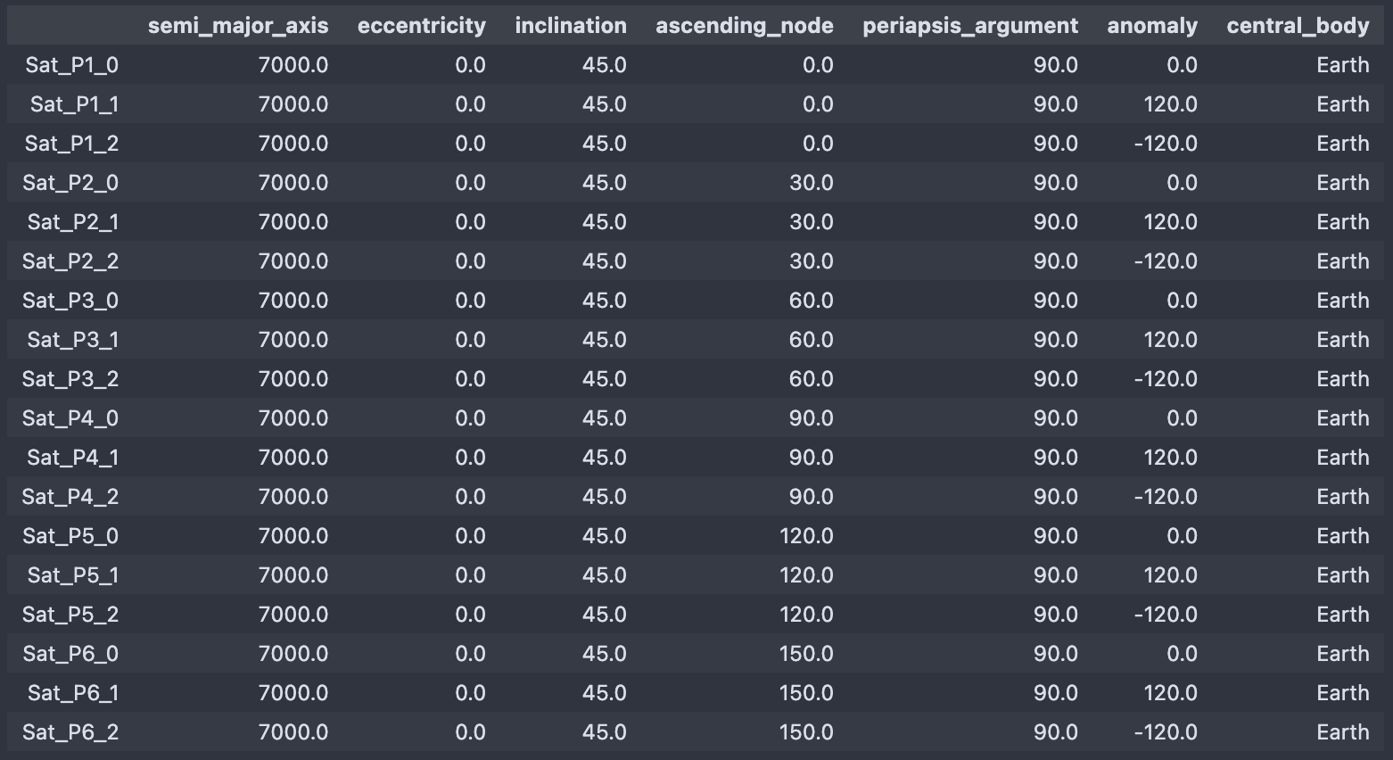
The satellites of the Walker star constellation
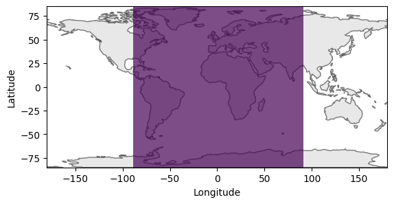
Next we load an area of interest (AOI) from a GeoJSON file.
import geojson_pydantic

with open("half_earth.geojson") as f:
    aoi = geojson_pydantic.FeatureCollection.model_validate_json(f.read())
Now we can set up the scenario with the constellation and the AOI.
Note
We are using the auto-discretization capabilites of Ephemerista here which use rectangles by default. If desired, a different discretization algorithm for a hexagonal grid based on H3 can be used. Disabling automatic discretization is also possible in which case the user needs to provide a list pre-discretized AOIs.
from ephemerista.constellation.design import Constellation
from ephemerista.scenarios import Scenario

start_time = Time.from_iso("TDB", "2016-05-30T12:00:00")
end_time = start_time + TimeDelta.from_hours(24)

scenario = Scenario(
    name="Coverage analysis with constellation",
    start_time=start_time,
    end_time=end_time,
    areas_of_interest=aoi.features,
    constellations=[Constellation(model=constel)],
    auto_discretize=True,
    discretization_resolution=5,
)
from ephemerista.analysis.coverage import Coverage

cov = Coverage(scenario=scenario)
results = cov.analyze()
fig = results.plot_mpl()
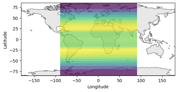
Coverage of the Walker constellation
Street-of-Coverage constellation
In this example we model the Iridum constellation to showcase the Street-of-Coverage constellations.
iridium = StreetOfCoverage(
    time=Time.from_iso("TDB", "2016-05-30T12:00:00"),
    nsats=66,
    nplanes=6,
    semi_major_axis=7158,
    inclination=86.4,
    eccentricity=0.0,
    periapsis_argument=0,
    coverage_fold=1,
)
## Inspect the Constellation
iridium.to_dataframe()
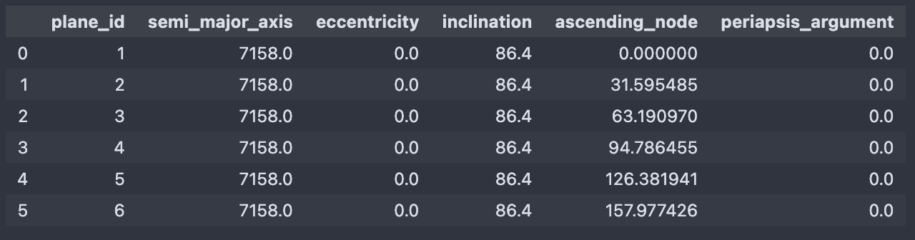
The planes of the Iridium constellation
## Investigate satellites
iridium.to_dataframe("satellites")
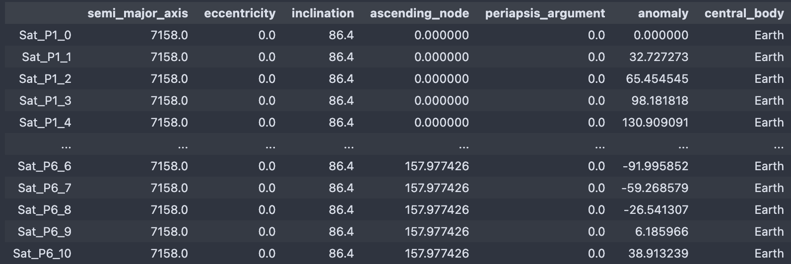
The satellites of the Iridium constellation
scenario_short = Scenario(
    name="Coverage analysis with constellation",
    start_time=start_time,
    end_time=start_time + TimeDelta.from_hours(2),
    areas_of_interest=aoi.features,
    constellations=[Constellation(model=iridium)],
    auto_discretize=True,
    discretization_resolution=5,
)
from ephemerista.analysis.coverage import Coverage

cov = Coverage(scenario=scenario_short)
results = cov.analyze()
fig = results.plot_mpl()
Coverage of the Iridium constellation
Which allows us to verify that the Iridium constellation successfully provides global coverage at all times.
Navigation
Navigation analysis evaluates GNSS-like systems. This section demonstrates:
Navigation constellation setup
Dilution of Precision (DOP) calculations
Navigation performance metrics
import ephemerista
from ephemerista.analysis.navigation import Navigation
from ephemerista.assets import Asset, GroundStation, Spacecraft
from ephemerista.propagators.sgp4 import SGP4
from ephemerista.scenarios import Scenario
from ephemerista.time import Time
To get a realistic example we are using a set of TLEs for the Galileo constellation but a custom constellation design could also be used. The observers of the GNSS constellation need to be defined as ground station assets.
with open("../tests/resources/navigation/galileo_tle.txt") as f:
    lines = f.readlines()

start_time = Time.from_components("TAI", 2025, 1, 27)
end_time = Time.from_components("TAI", 2025, 1, 28)

assets = [Asset(name="ESOC", model=GroundStation.from_lla(8.622778, 49.871111))]
for i in range(0, len(lines), 3):
    tle = lines[i : i + 3]
    name = tle[0].strip()
    assets.append(Asset(name=name, model=Spacecraft(propagator=SGP4(tle="".join(tle)))))

scenario = Scenario(start_time=start_time, end_time=end_time, assets=assets)
observer = scenario["ESOC"]
nav = Navigation(scenario=scenario).analyze()
nav.depth_of_coverage[observer.asset_id]
This will return the depth of coverage for a specific observer with a minimum of 13 and maximum of 17 satellites for this specific example.
nav.plot(observer.asset_id)
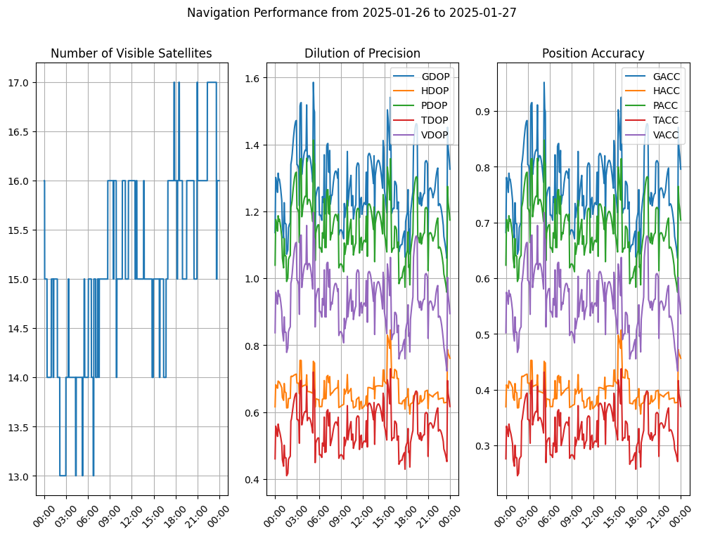
Navigation results
Next Steps
This manual covers the core functionality of Ephemerista. For more advanced usage:
API Documentation: See the complete API reference for detailed class and method documentation
Advanced Examples: Check the
examples/directory for additional specialized examplesCustom Analysis: Use the framework patterns shown here to build custom analysis workflows
Performance: For large-scale analysis, consider the parallel processing options available in the analysis modules
Troubleshooting
Common Issues
Data File Errors: Ensure EOP and ephemeris files are accessible and up-to-date
Memory Issues: For large constellations, use temporal sampling or parallel processing
Visualization Problems: Interactive plots require a Jupyter environment or compatible viewer
Getting Help
Check the API documentation for detailed method signatures
Look at the test files for additional usage patterns
Refer to the working notebook examples for complex workflows